Binary probit regression with I-priors
Department of Statistics PhD Presentation Event. London School of Economics and Political Science, 8-9 May 2017.
Abstract
An extension of the I-prior methodology to binary response data is explored. Starting from a latent variable approach, it is assumed that there exists continuous, auxiliary random variables which decide the outcome of the binary responses. Fitting a classical linear regression model on these latent variables while assuming normality of the error terms leads to the well-known generalised linear model with a probit link. A more general regression approach is considered instead, in which an I-prior on the regression function, which lies in some reproducing kernel Hilbert space, is assumed. An I-prior distribution is Gaussian with mean chosen a priori, and covariance equal to the Fisher information for the regression function. By working with I-priors, the benefits of the methodology are brought over to the binary case - one of which is that it provides a unified model-fitting framework that includes additive models, multilevel models and models with one or more functional covariates. The challenge is in the estimation, and a variational approximation is employed to overcome the intractable likelihood. Several real-world examples are presented from analyses conducted in R.
Keywords: binary, probit, regression, kernel, RKHS, Gaussian, process, multilevel, longitudinal, functional, prior, variational, Bayes, EM
Links
- Presentation slides - PDF
- Source code - GitHub
- R/iprior package - CRAN, GitHub
- R/iprobit package - GitHub
Main results
- Variational I-prior probit models in R
- Predicting cardiac arrhythmia
- Meta-analysis of smoking cessation
- Other supplementary material
Fisher’s Iris data set
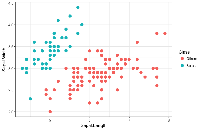
Varitional inference for I-prior probit models are implemented in the R package iprobit. A simple demonstratation is shown using the classical Fisher’s Iris data set, where the goal is to distinguish between the two classes (Setosa vs. Others).
Model fitting
R> system.time(
+   (mod <- iprobit(y, X))
+ )
##
## |=================================                     |  61%
##  Converged after 6141 iterations.
##  Training error rate: 0 %
##     user  system elapsed
##   67.857   6.396  74.277
Model summary
R> summary(mod)
##
## Call:
## iprobit(y = y, X, maxit = 10000)
##
## RKHS used: Canonical
##
##           Mean   S.E.    2.5%   97.5%
## alpha  -4.1730 0.0816 -4.3330 -4.0129
## lambda  1.2896 0.0142  1.2618  1.3175
##
## Converged to within 1e-05 tolerance. No. of iterations: 6141
## Model classification error rate (%): 0
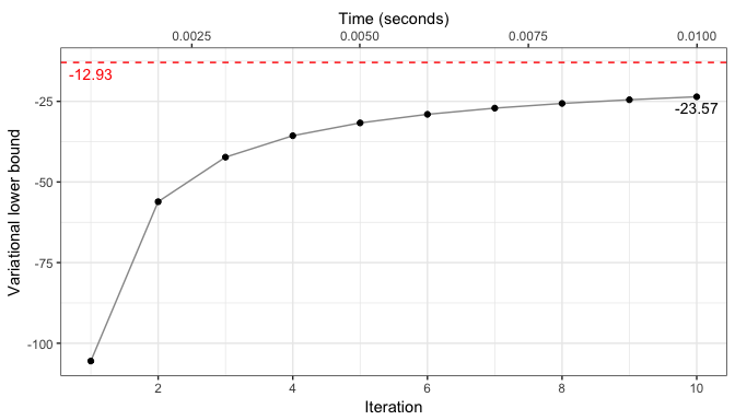
## Variational lower bound: -12.93486
Monitoring the lower bound
R> iplot_lb(mod, niter.plot = 10)
Decision boundary
R> iplot_decbound(mod)

Cardiac arrhythmia data set
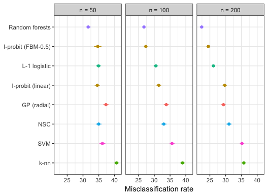
Distinguishing between the presence and absence of cardiac arrhythmia based on 194 predictors which includes various ECG data and other attributes such as age and weight. The out-of-sample prediction error is compared against various popular classififiers. The training sets were subsampled from the full data set, and the remaining data served as the validation set.
Results of experiments
The table shows the average misclassification rates (out of 100) and standard errors from 100 repetitions of the experiments. Ranking was done based on a simple weighted average across subsamples, with more weight given to small misclassification rates and small sub-samples.
| n = 50 | n = 100 | n = 200 | Rank | |
|---|---|---|---|---|
| I-probit (linear) | 34.54 (0.43) | 31.43 (0.38) | 29.72 (0.35) | 4 |
| I-probit (FBM-0.5) | 34.69 (0.59) | 27.28 (0.29) | 24.51 (0.30) | 2 |
| k-nn | 40.64 (0.33) | 38.94 (0.33) | 35.76 (0.36) | 8 |
| SVM | 36.16 (0.47) | 35.64 (0.39) | 35.20 (0.35) | 7 |
| GP (radial) | 37.28 (0.42) | 33.80 (0.40) | 29.31 (0.35) | 5 |
| Random forests | 31.65 (0.39) | 26.72 (0.29) | 22.40 (0.31) | 1 |
| NSC | 34.98 (0.46) | 33.00 (0.44) | 31.08 (0.41) | 6 |
| L-1 logistic | 34.92 (0.42) | 30.48 (0.34) | 26.12 (0.27) | 3 |
Plot of results
Meta-analysis of smoking cessation
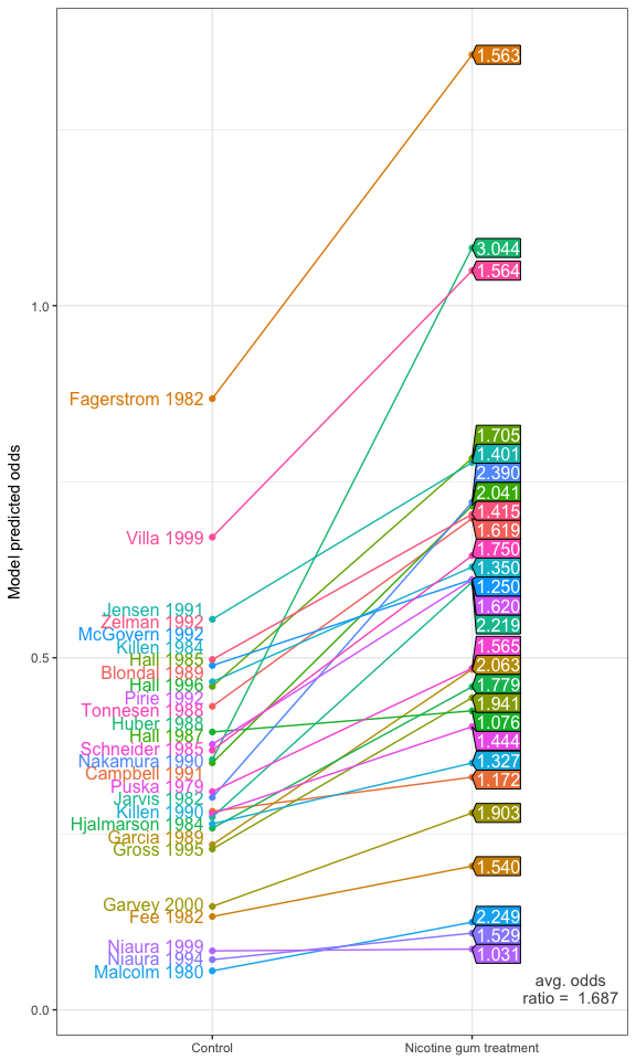
Estimating the treatment effect of nicotine gum to aid smoking cessation from a meta-analysis of 27 independent scientific studies.
Model comparison
Model 1 only considers treatment effect and ignores study-groups. Model 2 considers both treatment and study-group effects. Model 3 is similar to Model 2 with an addition of an interaction effect between treatment and study groups. Model 3 is the model chosen, as it implies the effectiveness of the treatments on quitting smoking varies across study groups.
| Model | Lower bound | Brier score | No. of RKHS param. | |
|---|---|---|---|---|
| 1 | f1 | -3210.79 | 0.0311 | 1 |
| 2 | f1 + f2 | -3097.24 | 0.0294 | 2 |
| 3 | f1 + f2 + f12 | -3091.21 | 0.0294 | 2 |
Notes: The Brier score measures the accuracy of probabilistic predictions.
Model predicted odds
Unlike logistic models, the fitted probabilities and hence the odds needed to be calculated manually. These, together with the naive 95% credibility interval, are tabulated below for each of the 27 studies.
| Study | Control | Treated | Odds ratio |
|---|---|---|---|
| Blondal 1989 | 0.43 (0.25, 0.58) | 0.70 (0.45, 1.01) | 1.62 (0.77, 4.10) |
| Campbell 1991 | 0.28 (0.17, 0.38) | 0.33 (0.17, 0.42) | 1.17 (0.44, 2.54) |
| Fagerstrom 1982 | 0.87 (0.57, 1.29) | 1.36 (0.96, 2.20) | 1.56 (0.74, 3.88) |
| Fee 1982 | 0.13 (0.06, 0.17) | 0.20 (0.10, 0.26) | 1.54 (0.60, 3.99) |
| Garcia 1989 | 0.23 (0.11, 0.29) | 0.48 (0.30, 0.68) | 2.06 (1.04, 6.44) |
| Garvey 2000 | 0.15 (0.06, 0.18) | 0.28 (0.15, 0.37) | 1.90 (0.87, 5.88) |
| Gross 1995 | 0.23 (0.10, 0.28) | 0.44 (0.26, 0.61) | 1.94 (0.94, 5.87) |
| Hall 1985 | 0.46 (0.26, 0.62) | 0.78 (0.51, 1.16) | 1.71 (0.83, 4.43) |
| Hall 1987 | 0.35 (0.18, 0.45) | 0.72 (0.48, 1.07) | 2.04 (1.06, 5.95) |
| Hall 1996 | 0.39 (0.25, 0.55) | 0.42 (0.23, 0.55) | 1.08 (0.41, 2.25) |
| Hjalmarson 1984 | 0.26 (0.13, 0.33) | 0.46 (0.28, 0.64) | 1.78 (0.84, 4.87) |
| Huber 1988 | 0.36 (0.16, 0.44) | 1.08 (0.80, 1.86) | 3.04 (1.83, 11.6) |
| Jarvis 1982 | 0.27 (0.13, 0.34) | 0.61 (0.40, 0.89) | 2.22 (1.17, 6.98) |
| Jensen 1991 | 0.55 (0.35, 0.79) | 0.78 (0.50, 1.13) | 1.40 (0.63, 3.27) |
| Killen 1984 | 0.47 (0.29, 0.65) | 0.63 (0.39, 0.89) | 1.35 (0.59, 3.10) |
| Killen 1990 | 0.26 (0.15, 0.35) | 0.35 (0.19, 0.46) | 1.33 (0.54, 3.07) |
| Malcolm 1980 | 0.06 (0.02, 0.06) | 0.12 (0.06, 0.15) | 2.25 (0.97, 9.11) |
| McGovern 1992 | 0.49 (0.31, 0.69) | 0.61 (0.37, 0.85) | 1.25 (0.53, 2.78) |
| Nakamura 1990 | 0.30 (0.14, 0.37) | 0.72 (0.49, 1.10) | 2.39 (1.31, 7.82) |
| Niaura 1994 | 0.07 (0.03, 0.09) | 0.11 (0.04, 0.13) | 1.53 (0.50, 4.12) |
| Niaura 1999 | 0.08 (0.05, 0.11) | 0.09 (0.02, 0.09) | 1.03 (0.21, 2.09) |
| Pirie 1992 | 0.38 (0.21, 0.50) | 0.61 (0.38, 0.87) | 1.62 (0.76, 4.12) |
| Puska 1979 | 0.28 (0.15, 0.37) | 0.40 (0.23, 0.54) | 1.44 (0.62, 3.49) |
| Schneider 1985 | 0.31 (0.17, 0.41) | 0.49 (0.29, 0.67) | 1.56 (0.71, 3.94) |
| Tonnesen 1988 | 0.37 (0.20, 0.48) | 0.65 (0.41, 0.93) | 1.75 (0.85, 4.65) |
| Villa 1999 | 0.67 (0.42, 0.96) | 1.05 (0.72, 1.63) | 1.56 (0.75, 3.87) |
| Zelman 1992 | 0.50 (0.30, 0.69) | 0.70 (0.44, 1.01) | 1.41 (0.64, 3.34) |
Plot of model predicted odds
Supplementary material
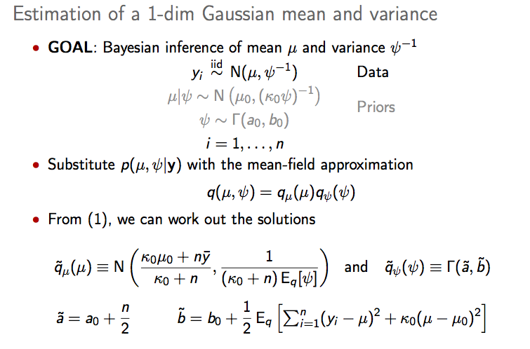
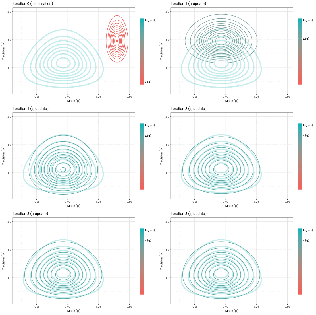
Variational inference for Gaussian mean and precision
Adapted from pp.31-32 of the presentation.
Copyright (C) 2017 Haziq Jamil. All rights reserved.